Videos
After some further consideration I think it's quite clear that the only probability mass function evaluated in the computation of  is that of the classically computed ideal distribution, denoted
  in the main paper.
This leads me to the conclusion that the phrasing of the following excerpt from section IV.C of the Supplemental Information (and especially the part underlined in red) is a bit unfortunate/misleading:
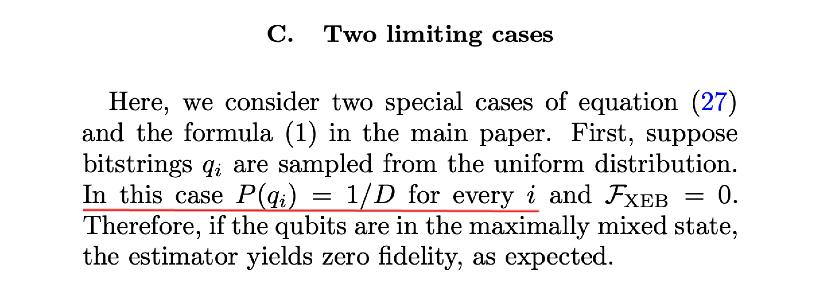
Just because the empirically measured bitstrings are coming from the uniform distribution doesn't mean that  is suddenly
  for all
  .
.  , as it goes into the calculation of the
  , is still the probability of sampling bitstring
  from the classically computed ideal distribution. This is in general not
  .
.
The correct reasoning is that the fact that  will be
  (and
(and  ) when bitstrings
  are sampled from the uniform distribution follows from the definitions of expectation and probability mass function:
The definition of expected value is the following sum
 where
where  is the probability of bitstring
  being sampled from the classically computed ideal quantum circuit,
  is the probability of
  being sampled from the non-ideal empirical distribution, and the sum runs over all possible bitstrings.
When bitstrings are coming from the uniform distribution  will always be
  so can be broken out of the sum:
 When you sum any probability mass function (of which
  is one example) over all the possible outcomes you by definition get 1, and thus:

That seems to restrict the output probability distributions of all quantum circuits to rather high entropy distributions.
The output of a typical randomly chosen quantum circuit is rather high entropy. That doesn't mean you can't construct circuits that have low entropy outputs (you can), it just means that picking random gates is a bad strategy for achieving that goal.
how can i
equal
when the bitstrings
are sampled from the uniform distribution?
How could it equal anything else? The probabilities of the target distribution have to add up to one, and you're picking each element  of the time. For example, if there was a single element with all the probability, you'd score
  . You always score
  on average when picking randomly.
How can the value of
correspond to "the probability that no error has occurred while running the circuit"?
When the paper says "the probability that no error occurs", what it means is "In the systemwide depolarizing error model, which is a decent approximation to the real physical error model at least for random circuits, the linear xeb score corresponds to the probability of sampling from the correct distribution instead of the uniform distribution.".
Physically, it is obviously not the case that either a single error happens or no error happens. For example, every execution of the circuit is going to have some amount of over-rotation or under-rotation error due to imperfect control. But that's all very complicated. To keep things simple you can model the performance of the system as if your errors were from simpler models, such as each gate have a probability of introducing a Pauli error or such as you either sample from the correct distribution or the uniform distribution.
Simplified models actually do a decent job of predicting system performance, particularly on random circuits. For example, consider the way the fidelity decays as the number of qubits and number of layers are increased. The fidelity decay curve from the paper matches what you would predict if every operation had some fixed probability of introducing a Pauli error.